
. INTRODUCTION
In optically stimulated luminescence (OSL) dating, the assessment of certain parameters of interest (i.e., De) is essential in estimating sample age. Routinely, a large set of aliquots (grains) are analyzed from which a single De (i.e., the characteristic De determined using a statistical model) is ultimately obtained along with its standard error estimate. Galbraith and Roberts (2012) reviewed the most commonly used statistical age models in determining the characteristic De, namely, from the simple central age model (CAM) (Galbraith et al., 1999) to more sophisticated ones, such as the minimum age model (MAM) (Galbraith et al., 1999).
Maximum likelihood estimation (MLE), which provides point estimates of parameters and associated standard errors, is routinely adopted to estimate parameters used in these statistical age models by maximizing the logged-likelihood function (Galbraith et al., 1999; Galbraith and Roberts, 2012). The burial age is obtained by dividing the characteristic De estimated using MLE by the average environmental dose rate of the sample, and the associated standard error is estimated using propagation of error formulas (referred to as the standard approach). However, the standard approach only provides a coarse characterization of the statistics associated with burial age. Moreover, it does not permit the inclusion of additional information, such as order constraints between the ages of a given stratigraphic sequence to improve age estimates (Combès and Philippe, 2017).
In contrast, the Markov chain Monte Carlo (MCMC) methods construct a Markov chain while converging to the desired sampling distribution by starting from random initials and seeking to characterize posterior distributions for parameters of interest (Gelman et al., 2014). Furthermore, MCMC methods treat model parameters as full probability distributions and produce samples from the joint posterior density of parameters that are then summarized for the purpose of Bayesian inference. By doing so, the uncertainty over the range of potential parameter values is also estimated, rather than only a single point estimate (Annis et al., 2017). Summary statistics (such as the mean, the median, the standard deviation, the confidence interval, etc.) are obtained directly from randomly generated samples.
Such MCMC methods have increasingly been employed to analyze OSL data for Bayesian inferences (e.g., Millard, 2004; Sivia et al., 2004; Huntriss, 2008; Zink, 2013, 2015; Peng and Dong, 2014; Combès et al., 2015; Cunningham et al., 2015a, 2015b; Guérin et al., 2015; Mercier et al., 2016; Peng et al., 2016a; Christophe et al., 2018; Philippe et al., 2019). For example, Sivia et al. (2004) used an MCMC method to analyze the finite mixture age mode (FMM) (Galbraith and Green, 1990; Roberts et al., 2000) as well as a noised FMM using unlogged De sets. Cunningham et al. (2015a, 2015b) developed an age model to account for effects of variation in aliquot size and luminescence sensitivity on partially-bleached De distributions while using an MCMC method to obtain the posterior of parameter estimates. Combès et al. (2015) proposed a hierarchical model to describe the central De for fully bleached aliquots (grains). A Metropolis-within-Gibbs sampler is used to obtain the posterior of the characteristic dose. The model has been further expanded to analyse poorly bleached samples using a Gaussian mixture model (e.g., Christophe et al., 2018). Peng et al. (2016a) used a Slice-within-Gibbs sampling algorithm to obtain the posterior distribution of parameters in statistical age models reviewed by Galbraith and Roberts (2012). However, this model did not take into account the posterior distribution for burial age.
The first objective of this study is to estimate statistical model parameters (such as the CAM, the MAM, etc.) and obtain the posterior distribution for burial age through MCMC sampling under a Bayesian framework, using a combination of aliquot-level (grain-level) dose and sample-level dose-rate datasets. The burial dose and age estimated by MCMC are then compared with those estimated using the standard approach (i.e., MLE).
Bayesian models utilize stratigraphic relationships between samples to increase the precision of dates and to provide a sophisticated protocol to combine multiple age estimates into a meaningful chronological framework (Ramsey, 1995, 2008). By incorporating the stratigraphic principle that shallower sediments in the stratum sequence are younger than deeper sediments into age-depth models, Bayesian inference can reduce the uncertainty of dates wherein age probability distributions overlap. Age-depth modelling using Bayesian inference was initially developed to analyze radiocarbon dating data (Ramsey, 1995; Bayliss and Ramsey, 2004). Over the past decade, the application of Bayesian inference to model depth-age relationships using luminescence data have also gained widespread usage (e.g., Rhodes et al., 2003; Cunningham and Wallinga, 2012; Lanos and Philippe, 2015; Combès and Philippe, 2017; Zeeden et al., 2018; Tamura et al., 2019).
During the routine application of statistical age models, such as the CAM and MAM, characteristic De values of individual samples are estimated separately (e.g., Schmidt et al., 2012; Arnold et al., 2009), even when samples are collected from different depths in the same profile sequence (e.g., Arnold et al., 2007; Kunz et al., 2013; Peng et al., 2016b) and when age-depth relationship between samples may have been used as additional information to improve date estimates. Brill et al. (2015) applied statistical age models (including CAM and MAM) to obtain luminescence age estimates (and associated standard errors) for samples collected from a number of depositional sequences, and they used the age-depth modelling program OxCal to improve the accuracy and precision of these ages by making use of their relative stratigraphic order. However, this two-step protocol that consists of calculating burial ages using a standard approach and further perfect these age estimates using Bayesian inference may fail in characterizing distributions of interest because it decomposes the global inference into a two-step assessment that is likely to lead to a significant loss of information during each step in the process (Combès et al., 2015). Cunningham and Wallinga (2012) employed a bootstrap likelihood protocol to obtain the distribution of the characteristic De for a sequence of young fluvial samples using an unlogged version of the MAM. The replicate characteristic De values obtained by bootstrapping are used to construct a probability density function for each sample in order to apply Bayesian inference to improve OSL chronologies. However, as reiterated by Cunningham and Wallinga (2012), the boot-strap likelihood protocol is just an analogue of the likelihood function and does not produce a true likelihood.
The second objective of this study is to apply statistical age models to refine age-depth relationships using De datasets from multiple luminescence samples employing an alternative Bayesian inference model. In contrast to the method by Cunningham and Wallinga (2012), in this study characteristic De values are sampled directly from the probability density function that describes the statistical model (see the following section for more detail) through MCMC sampling. The joint probability density function for multiple OSL ages is constructed by utilizing a combination of statistical models and measured De and dose rate datasets. Both the CAM and MAM are used to flexibly analyze fully and partially bleached OSL dates, respectively, using MCMC in order to combine different types of statistical age models in a mathematically rigorous, geologically reasonable, and philosophically satisfying manner. The performance of the model is then tested on measured and simulated De distributions.
. A BRIEF INTRODUCTION TO GALBRAITH’S STATISTICAL AGE MODELS
The central age model (CAM)
Galbraith et al. (1999) recommended using the CAM to provide a representative estimate of the characteristic dose for samples that have not been affected by partial bleaching or sediment mixing. The benefit of the CAM is that it can take any over-dispersion (OD) into account when estimating the weighted mean dose and its standard error (Galbraith and Roberts, 2012). OD provides an estimate of the degree of dispersion that represents the relative spread in the De distribution that remains after allowing for measurement uncertainties. Routinely, OD is calculated as a descriptive statistic to reveal sources of variability in De (e.g., Thomsen et al., 2005; Jacobs et al., 2006). The OD of De distributions in well-bleached analogues is commonly used as an input for statistical age models when analyzing measured sedimentary samples (Galbraith and Roberts, 2012). The likelihood function of the CAM can be described as follows:
where yj and xj represent for the jth logged De value and its relative standard error (RSE), respectively. p(Dj|θ) represents the probability of data Dj given parameter θ. μ and σ represent the parameters of interest (i.e., the logged characteristic De and the OD, respectively).Optimal parameters can be obtained using either an iterative numeric procedure or by direct numerical maximization of the joint-likelihood determined from paired observations D={xj, yj | j=1,2,3,...,n) (Galbraith et al., 1999). Most free and commercial optimization environments (such as R, Matlab, etc.) provide well-designed optimization routines for optimization usage. The standard errors of parameters are conventionally obtained by inverting the Hessian matrix estimated by finite-difference approximation.
The minimum age model (MAM)
One of the most widely used statistical models for tackling partially-bleached samples is the MAM (Galbraith et al., 1999; Galbraith and Roberts, 2012), which is based on well-established statistical principles. In this model, true logged characteristic De value is assumed to be drawn from a truncated Normal distribution, and the lower truncation point (i.e., γ) represents the mean of the logged characteristic dose of fully bleached grains. Two versions of the model are available, namely, the 3-parameter minimum age model (MAM3) and its 4-parameter counterpart (MAM4). The properties of the dataset (i.e., the degree of dispersion, the number of data points, the uncertainties associated with De values, etc.) may strongly affect the quality of the estimate in the application of the MAM4 (Galbraith and Roberts, 2012). In contrast, the MAM3 usually works well even for lowly dispersed De sets, while also being rather numerically stable compared to the MAM4.
Galbraith et al. (1999) noted that some datasets, particularly those with small numbers of De values or less dispersed distributions, do not warrant fitting with the MAM4, and that a more robust estimate of the characteristic dose may be obtained using the MAM3. Consequently, the MAM3 is conveniently regarded as the “default” model (Arnold et al., 2009) and has been widely applied in the literature to determine burial dose (e.g., Arnold et al., 2007; Schmidt et al., 2012; Kunz et al., 2013). According to Galbraith et al. (1999), the likelihood function of the MAM3 can be described as follows:
whereThree quantities (p, μ, and σ) must be optimized in this model. p denotes the proportion of grains that are fully bleached before burial, μ denotes the logged characteristic dose, and σ is an adjustable parameter used to account for the dispersion in partially bleached grains (in unit per cent). Note that, conventionally, the logged characteristic dose in the MAM3 is represented by γ, and in this study μ is alternatively used to make it correspond to that which is in the CAM. Φ(x) denotes the standard Normal cumulative distribution function. The optimal parameters are typically estimated by direct numerical maximization of the joint-likelihood that is determined using paired observations D={xj, yj | j=1,2,3,...,n). In contrast to the CAM, optimization of the MAM3 is considered an ill-conditioned mathematical problem due to the strong nonlinearities in the calculation. Whether it is possible to converge it to global optimal estimates depends heavily on the choice of the initial parameters used. It is indispensable to try various initial parameter sets to obtain optimal estimates.
The maximum age model (MXAM)
The maximum age model (MXAM) is an analogue of the MAM and is firstly applied by Olley et al. (2006) in their estimation of the maximum dose population from De distributions. Galbraith and Roberts (2012) enumerated two scenarios where the MXAM is applicable: (1) Samples composed of fully bleached grains that have subsequently been mixed with younger, intrusive grains, and (2) samples composed of fully bleached grains, some proportion of which have been bleached after deposition.
The characteristic dose of the MXAM3 can be estimated according to the MAM3 by using a “mirror image” of the original De distribution as an input (Olley et al., 2006; Galbraith and Roberts, 2012). Alternatively, by accounting for the fact that the lower truncation point of a truncated Normal distribution denotes the minimum characteristic dose in the MAM3 while the upper truncation point of a truncated Normal distribution denotes the maximum characteristic dose in the MXAM3, the likelihood for the MXAM3 can be derived by a minor modification of Eq. 2.2 and can be described as follows:
where μ0 and σ0 are calculated in the same manner as the corresponding values in the MAM3.Unlogged versions of statistical age models
Larger De estimate typically have larger absolute standard errors; namely, larger De estimates will vary more (Arnold and Roberts, 2009). Consequently, the frequency distribution of De estimates will tend to be positively skewed. The Lognormal distribution provides a simple model to describe variables wherein their standard deviations increase in proportion to their means. It is for this reason that the aforementioned statistical age models use log-transformed De datasets as inputs. Datasets in log-scale are obtained by calculating natural logarithms of De estimates and transforming their absolute standard errors into RSEs. This is because the RSE of a De estimate approximates the standard error of a De estimate on a natural logarithm scale (Galbraith and Roberts, 2012). As a result, these statistical age models are unsuitable for measured zero or negative De values that are consistent with zero or positive De values within a level of uncertainty. However, such types of De distribution are frequently encountered for either very young or modern samples. As a consequence, Arnold et al. (2009) used unlogged versions of the CAM and the MAM to analyze young/modern De datasets using a series of known-age fluvial samples and demonstrated that the unlogged versions of these models are capable of producing accurate burial dose estimates from their samples. To apply un-logged versions of these models, the user needs only use the original De values and their absolute standard errors as yjs and xjs, respectively, in Eqs. 2.1–2.3. In this case, the estimated μ denotes the characteristic dose (not the logged counterpart), while σ denotes a parameter in unit Gy (not in per cent).
. ANALYZING GALBRAITH’S STATISTICAL AGE MODELS USING MCMC
MCMC sampling from statistical age models for individual samples
The statistical age models described in Section 2 are in fact equivalent dose models. This is because they estimate the characteristic De instead of the burial age (e.g., Guérin et al., 2017). However, they can be easily transformed to obtain the posterior distribution of ages by taking the dose rate data into consideration during the simulation process:
where a denotes the age, μ denotes the characteristic dose,Each parameter is assigned a prior distribution that represents the prior knowledge of it before some evidence is considered. For p (i.e., the proportion of fully bleached grains), a Uniform prior that lies between 0.001 and 0.999 was used. For a (i.e., burial age) a typically employed non-informative prior is a Uniform distribution with lower and upper bounds set to equal amin and amax, which specifies a particular period of the burial history (e.g., Combès and Philippe, 2017). Parameter σ (i.e., a scale parameter inside the model) is an adjustable parameter that captures the unknown spread within the whole De distribution (for the CAM) or only the unknown spread in the De distribution for partially bleached grains (for the MAM3). A significant amount of variation in OD exists between samples that either have different inherent luminescent properties, undergo different burial histories, and those that have been affected by various factors related to variation in microdosimetry and uncertainty from the measurement procedure. A summary of OD values from sedimentary samples (some are thought to have been fully bleached at the time of deposition) in published studies reveals that single-grain De distributions exhibit OD values of up to 30% (or higher), and the De distributions of multi-grain aliquots have a mean OD of 14% (Arnold and Roberts, 2009). OD values for several partially bleached young/modern fluvial samples calculated using an unlogged CAM range from 24% to 208% (Arnold et al., 2009). In this study, the prior of σ was represented using a Uniform distribution over the interval (0, 5).
Galbraith and Roberts (2012) reiterated that an estimate of additional uncertainty (σb) should be added in the quadrature to the RSE of each De value before running the MAM (as well as the MXAM) (Galbraith et al., 2005). σb represents the underlying spread in dose distribution typically present in well-bleached and undisturbed samples. An overestimate of σb will lead to an overestimate of the characteristic dose (and hence the burial age), and vice versa. Ideally, σb should be calculated from a well-bleached sample of the same mineral derived from the same source and, also ideally, of equivalent age (Galbraith and Roberts, 2012). In the absence of such information, σb values of 10% and 20% could be coarse approximations at multiple-grain and single-grain levels, respectively (e.g., Arnold and Roberts, 2009).
MCMC sampling from statistical age models for multiple samples with order constraints
In this section, an age-depth model to combine De datasets from multiple samples with stratigraphic constraints was considered by using the statistical age models described in Section 2. Although Bayesian age-depth models are expected to improve the precision of dates, such precision may be misleading if potential systematic uncertainties have not been included by the individual samples (Zeeden et al., 2018). Compared to the application of statistical age models to individual samples using the standard approach, incorporating statistical age models into a Bayesian age-depth framework to refine the age-depth relationship between dates from multiple samples with order constraints requires that both random and systematic sources of errors are properly accounted for; otherwise, the precision of dates may increase decisively in unjustified ways (Combès and Philippe, 2017; Zeeden et al., 2018).
This study adopted the method described by Combès and Philippe (2017) to build the relationship between the characteristic dose μi, the annual dose rate
For parameters pi and σi of the ith sample (i=1, 2, 3, ..., N), the priors were set equal to p and σ, respectively. For parameter ai, a Uniform distribution for which the lower and upper bounds were set equal to amini and amaxi was used (the same as Section 3 – MCMC sampling from statistical age models for individual samples). In addition, a constraint on vector [a1, a2, a3, ..., aN] such that a1<a2<a3<...<aN (i.e., wherein ages are sorted in ascending order) was imposed to allow stratigraphic information to be incorporated during the MCMC sampling process.
Stan (programming language) implementation for MCMC sampling
The objective being to obtain sampling distributions of parameters p(θ|D) based on the joint-likelihood p(D|θ) and priors p(θ) using MCMC sampling, a class of algorithms that utilize Markov chains to allow for the approximation of posterior distributions for parameters of interest by utilizing the prior distributions and likelihood as inputs (Annis et al., 2017). This study adopted the recently developed software package Stan (Gelman et al., 2015) for this purpose. Although there are dozens of built-in probability distributions that can be used to sample standard distributions (such as the Normal distribution, the Exponential distribution, etc.), users will occasionally require “non-standard” distributions (i.e., the joint-likelihoods for the CAM, MAM3, and MXAM3 used in this study) that may not yet be defined. Annis et al. (2017) gave a detailed tutorial on the implementation of MCMC sampling using user-defined distributions within the Stan programming language. Once the user-supplied function is defined, it can be called upon as a built-in distribution. This section provides a simple description of the numeric programs used to conduct MCMC sampling from statistical age models applying De datasets from both individual and multiple samples using the Stan software package. The relevant code and numeric scripts are freely downloadable from https://github.com/pengjunUCAS/mcmcSAM.
Individual samples
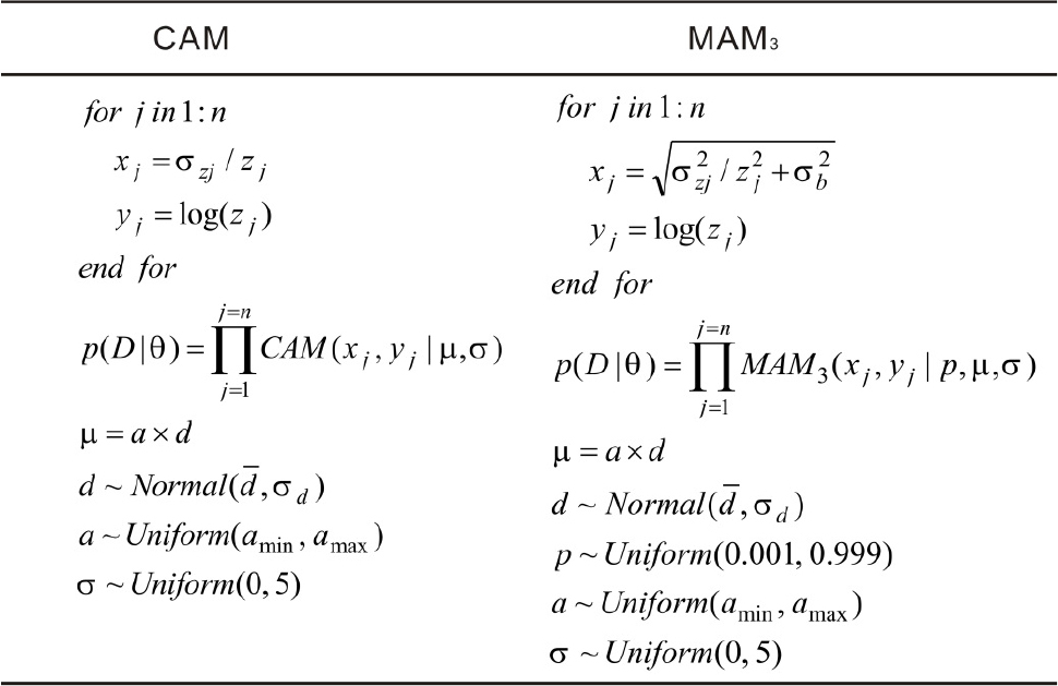
The input, likelihood, transformation, and distribution used to implement MCMC sampling for individual samples using the CAM and the MAM3 are illustrated in Fig. 1. The MXAM3 can be simulated in the same manner as the MAM3 by changing the likelihood correspondingly. In Fig. 1, zj and σzj denote the De and associated absolute error for the jth aliquot (grain). These statements can easily be modified to accommodate unlogged versions of the CAM, MAM3, and MXAM3. In Stan, variable definitions, distribution specifications, and program statements are placed within code blocks (Annis et al., 2017). Script “SAM0.stan” was employed to place all code blocks used to implement the sampling process. The R package “rstan” (an R interface for Stan) (Stan Development Team, 2018) was used to execute the script using a wrapper function mcmcSAM() available in the file “SAM.R”. Once the sampling process is terminated, the resultant MCMC convergence diagnostics are automatically stored in the file “mcmcSAM.pdf”, and the posterior samples are stored in the file ”mcmcSAM.csv”. Both files are available from the current R working directory. Please refer to the file “SAM.R” for more detail on arguments and default settings used in function mcmcSAM().
Multiple samples with order constraints
Samples from the same sequence may substantially vary in De distributions due to differences in provenance, depositional environment, microdosimetry, etc. There is no generally applicable statistical age model that can be used to analyze all De distribution types. If we conceptualize three samples (S1, S2, and S3) from the same stratigraphic sequence with their sample depths in ascending order, and we assume that these samples exhibit significantly different De distribution characteristics for which the most suitable models for these samples would be the MAM3, CAM, and MXAM3, respectively, then the statements used to conduct MCMC sampling on these samples applying a combination of different age models in log-scale can be summarized as shown in Fig. 2. zij and σzij denote the De and the associated absolute standard error for the jth aliquot (grain) from the ith sample. yij and xij denote the logged De and corresponding RSE for the jth aliquot (grain) from the ith sample. n1, n2, and n3 denote the numbers of aliquots (grains) for the three samples. p(D|θ) is calculated as the product of joint likelihoods for samples S1, S2, and S3 that are fitted using the MAM3, CAM, and MXAM3, respectively. Note that in this study only three samples are used for illustrative purposes, while in practice many samples fitted using various combinations of the three different age models can be simultaneously analyzed in a manner similar to that demonstrated in Fig. 2. This allows the programs to have a degree of flexibility when De distributions from the same sequence need to be treated differently. Two scripts (i.e., “SAMseq0.stan” and “SAMseq1.stan”) were used to conduct the sampling process without and with order constraints, respectively. A wrapper function mcmcSAMseq()that is available in file “SAMseq.R” was used to call these scripts. The resultant MCMC convergence diagnostics are automatically stored in file “mcmcSAMseq.pdf”, and the posterior samples are stored in file “mcmcSAMseq.csv”.
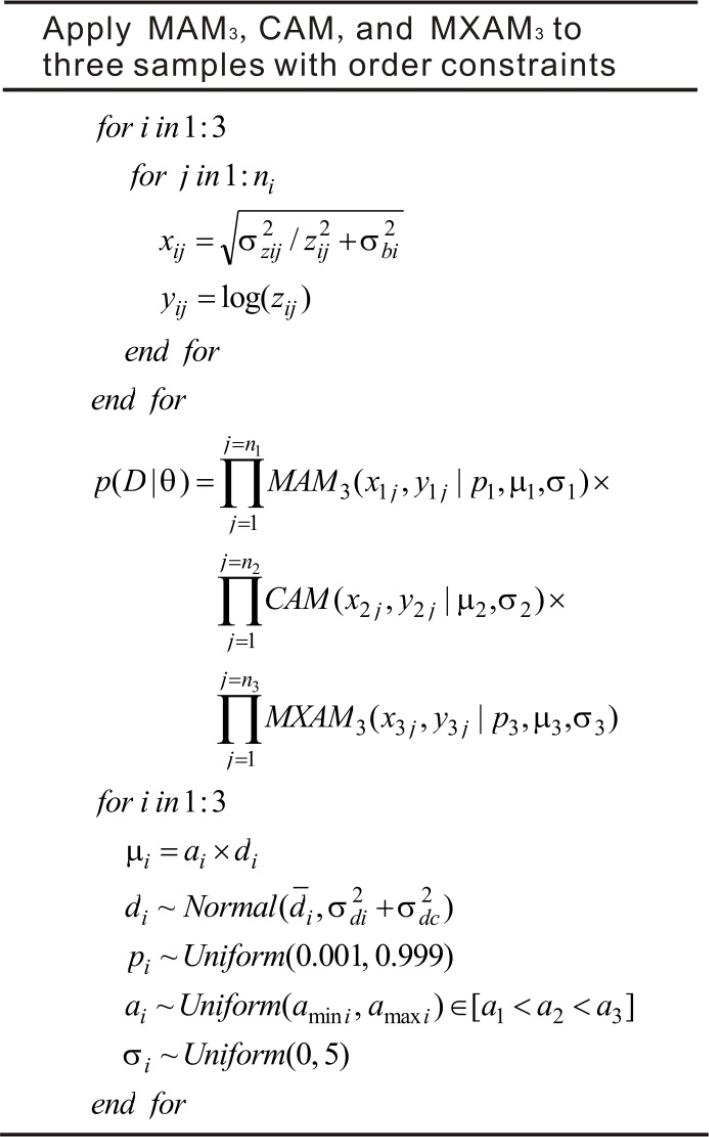
Fig. 2
Statements used for conducting MCMC simulation simultaneously according to different age models (log-scale) using De sets from three samples whose ages were constrained such that a1<a2<a3. The three samples were analyzed using the MAM3, CAM, and MXAM3, respectively. The protocol can be easily adapted for MCMC sampling without order constrains for burial ages.
. APPLICATIONS AND RESULTS
Measured De sets
First, the validity of the MCMC sampling protocol (as demonstrated in Fig. 1) used to analyze De sets from individual samples was checked using measured multi-grain De distributions (Fig. 3) of four aeolian samples (i.e., GL2-1 to GL2-4) from Gulang County at the southern margin of the Tengger Desert, China (Peng et al., 2016b). The De distributions were obtained using the single aliquot regenerative-dose (SAR) protocol (Galbraith et al., 1999; Murray and Wintle, 2000). When applying the MAM3 and MXAM3, an additional uncertainty (i.e., σb) of 10% was added in the quadrature to the RSEs of the measured De values to account for unrecognized measurement errors. In this study (unless stated otherwise), three parallel Markov chains (the number of iterations for each chain was set equal to 10000) were simulated during the MCMC sampling process for the individual samples, and four parallel Markov chains (the number of iterations for each chain was set equal to 6000) were simulated during the MCMC sampling process for the multiple samples. The lower and upper bounds for the priors of ages were set equal to amin(amini)=1 ka and amax(amaxi)=100 ka, respectively. The characteristic dose (i.e., μ) and age (i.e., a) of the CAM, MAM3, and MXAM3 obtained using MLE and MCMC were then compared and the results summarized in Table 1. The estimates obtained between the two different methods were consistent within errors, suggesting that estimates derived from MCMC can be used as an informative comparison for those estimated by MLE.
Fig. 3
Measured multi-grain De distributions for four aeolian samples from Gulang County at the southern margin of the Tengger Desert, China (Peng et al., 2016b). N denotes the number of measured aliquots. Note that in Peng et al. (2016b) an additional uncertainty of σb=5% was added in the quadrature to the RSEs of the measured De values to account for sources of errors that were not considered in the measurements. However, no additional uncertainty was added to the De distributions shown here.
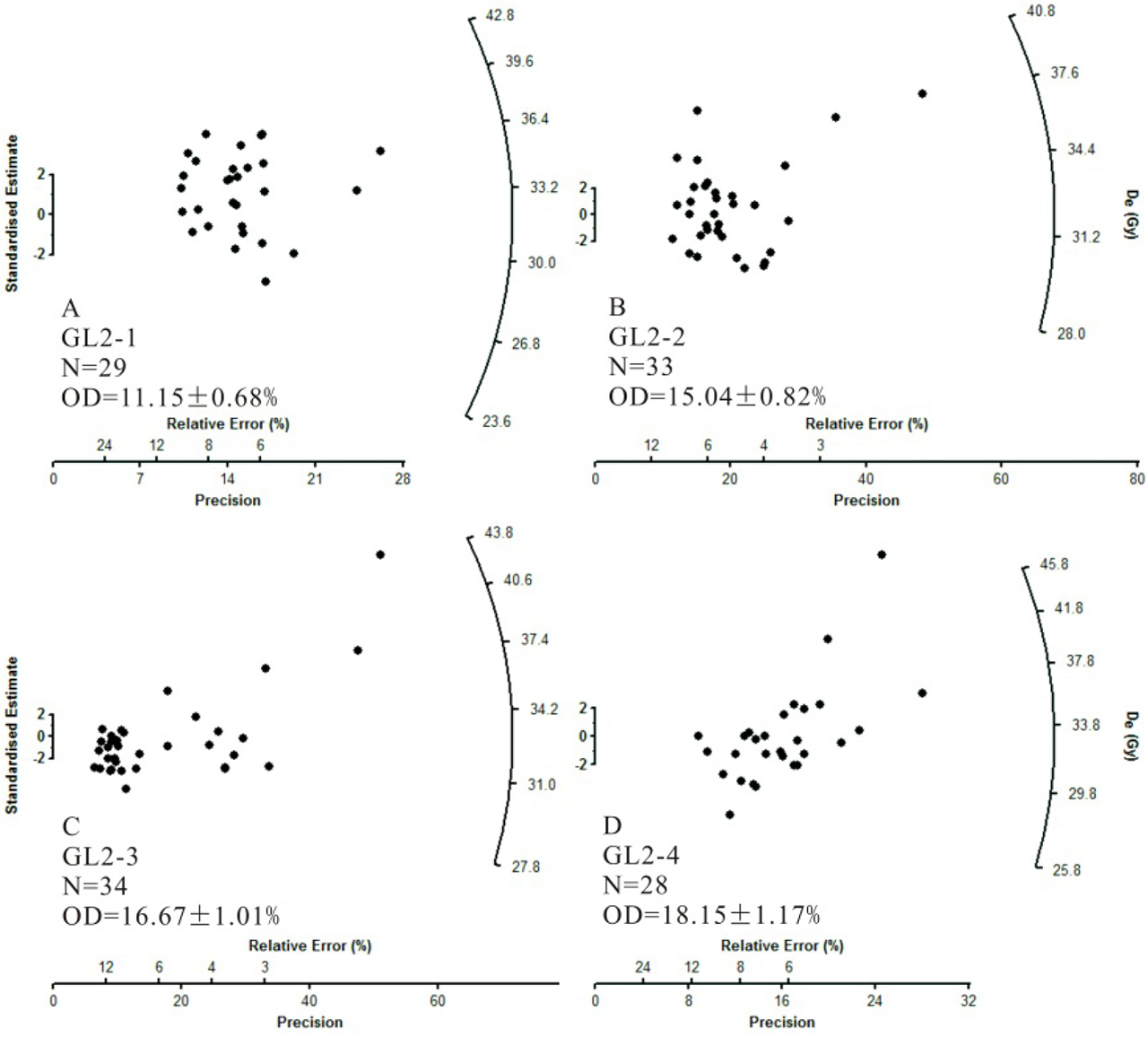
Table 1
Comparisons of burial dose and age estimated from MLE and MCMC for the various statistical age models using De sets from four measured aeolian samples. Quantities estimated using the MCMC sampling protocol shown in Fig. 1 are marked in bold. Quantities estimated using the MLE are inside parentheses.
These four samples were also analyzed simultaneously using the MCMC sampling protocol (as demonstrated in Fig. 2) for multiple samples. De values of these samples fell within reasonably narrow ranges and displayed homogeneous distributions (Fig. 3). Accordingly, the CAM was applied to determine the burial dose. Samples GL2-1, GL2-2, GL2-3, and GL2-4 were collected from the same section in ascending order depths. Consequently, their burial ages were also expected to be in ascending order. The MCMC sampling protocol was applied to these samples with order constraints (results shown in Table 2). The systematic error representing the error in the calibration of the dose rate measurement device shared by all samples was assumed to be σdc=0.1. The posterior distributions of burial age are shown in Fig. 4. Results obtained without order constraints were also provided for comparison. These results suggested that burial ages would be internally consistent with the stratigraphy if order constraints were imposed during the MCMC sampling process. Moreover, the posterior standard deviations of burial ages would be significantly reduced when using stratigraphic constraints, implying that the precision of burial ages improved. Finally, a comparison between Table 1 and Table 2 for CAM results demonstrated that burial dose and ages (and their posterior standard deviations) obtained by MCMC sampling using both individual samples and multiple samples simultaneously without order constraints were indistinguishable from each other.
Fig. 4
Posterior distributions of burial ages obtained from the CAM for the four aeolian samples taken from the same sedimentary section obtained using the MCMC sampling protocol, as shown in Fig. 2. The blue-coloured density plots denote results obtained by constraining the burial ages in ascending order. The grey-coloured density plots denote results obtained by imposing no constraints on the order of burial ages. The value inside parentheses denotes the calculated RSD of burial age.
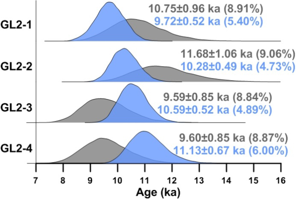
Table 2
A summary of burial dose and age estimated from the CAM for De sets from four measured aeolian samples using the MCMC sampling protocol shown in Fig. 2 without and with order constraints. The systematic error for the dose rate measurement shared by all samples was set to σdc=0.1.
Simulated De sets
This section shows simulation results of a series of De distributions with known burial ages to further verify the performance of the MCMC sampling protocols. The first three samples (#1–#3) were assumed to be partially-bleached, the next three samples (#4–#6) fully-bleached, and the last three samples (#7–#9) contain fully-bleached grains that have been subsequently mixed with younger, intrusive grains. These samples were assumed to be collected from the same sedimentary sequence but at different depths. Their “true” burial doses ranged from 18 to 42 Gy with a step of 3 Gy, and their “true” burial ages ranged from 7 to 11 ka with a step of 0.5 ka. The “true” average dose rate can be obtained by dividing the “true” burial dose by the “true” burial age of a sample. The random error arising from dose rate measurement was assumed to be 7%, in order to simulate a realistic annual dose rate. Namely, the “true” dose rates are noised using a Normal distribution with a mean equivalent to the “true” average dose rate and a relative standard deviation (RSD) equal to 7%. The generated random dose rates were used as the measured dose rates when determining burial ages using MLE and MCMC. The systematic error representing the error in the calibration of the dose rate measurement device shared by all samples was assumed to be zero (i.e., σdc=0).
Lognormal distributions were used to model the natural dispersion in dose distributions arising from dose rate variation with an RSD of 5% (i.e., σd=0.05). Measured De distributions were simulated according to the method described by Li et al. (2017), which involves simulating OSL intensities of the natural dose (Ln), a series of regenerative doses (Lx), and their corresponding test doses (Tn and Tx). Measured OSL sensitivity data taken from an empirical sample was used as the basis of the simulation. The OSL sensitivity (e.g., counts per unit of dose) of the different grains were randomly generated from a Gamma distribution fitted to the single-grain Tn datum from a sample taken from Lake Mungo, Australia (Fig. 5). Noise was added to each of the simulated OSL signal intensities based on the uncertainty arising from counting statistics and instrumental irreproducibility. It was assumed that both photon counts and dark counts were over-dispersed compared to a Poisson distribution (e.g., Li, 2007; Adamiec et al., 2012) and follow Negative Binomial distributions (e.g., Bluszcz et al., 2015). The variance to mean ratios for the photon counts and dark counts were set equal to 1.38 and 1.85, respectively. The dark count was set equal to 10 cts/0.2s. The instrumental reproducibility was set as 2%. For the natural signals (Ln), an extra noise from “intrinsic OD” (e.g., σm=10%), which represents unrecognized measurement errors (e.g., OD observed from a dose recovery experiment) (e.g., Thomsen et al., 2005; Jacobs et al., 2006; Guérin et al., 2017), was also added. De estimation was conducted using the R package “numOSL” (Peng et al., 2013; Peng and Li, 2017). For each sample, 100 De values (and associated errors) were simulated. The nine simulated De distributions are shown in Fig. 6.
Fig. 5
Distribution of OSL sensitivity for the 127 grains of a sample taken from Lake Mungo, Australia. The red line denotes the probability density curve obtained by fitting the OSL sensitivity data using a Gamma distribution. The fitted Gamma distribution has a shape parameter of α=0.565 and a rate parameter of β=0.191. Q[x%] denotes the x% sample quantile of OSL sensitivity.
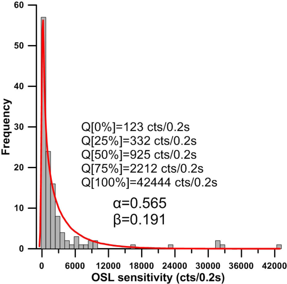
Fig. 6
Simulated De distributions of nine samples from a sedimentary sequence. Each De set contains 100 De values (and associated standard errors). The shaded bars in each plot indicate the burial dose within 2σ error. The first three samples (#1–#3) are partially-bleached, the next three samples (#4–#6) are fully-bleached, and the last three samples (#7–#9) contain fully-bleached grains that have been subsequently mixed with younger, intrusive grains. The nine samples are assumed to be collected from the same section but at different depths, and their estimated burial dose and age are summarized in Fig. 7 and Table 3.
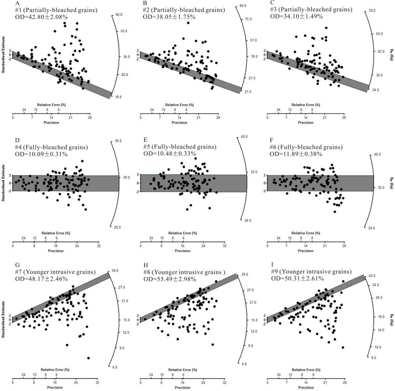
The simulated De sets were analyzed individually using MLE, analyzed simultaneously using MCMC without order constraints, and analyzed simultaneously using MCMC with order constraints. The first, next, and last three samples were analyzed using the MAM3, CAM, and MXAM3, respectively. To facilitate the model in the analysis of the MAM3 and the MXAM3, a σb should be determined beforehand. The calculated OD values for samples #4–#6 can be regarded as appropriate σb values, given that these samples are “fully-bleached” simulated samples whose errors, arising from dose rate variation (i.e., σd) and unrecognized measurement uncertainty (i.e., σm), were the same as samples #1–#3 and samples #7–#9. The estimated OD values were 10.09±0.31%, 10.48±0.33%, and 11.89±0.38%, respectively, for samples #4–#6. These values are broadly consistent with the expected value of
Fig. 7
Posterior distributions of burial ages of the nine simulated samples from a sedimentary section obtained using the MCMC sampling protocol, as shown in Fig. 2. Samples #1–#3, #4–#6, and #7–#9 were analyzed using the MAM3, CAM, and MXAM3, respectively. The blue-coloured density plots are results obtained by constraining burial ages in ascending order. The grey-coloured density plots are results obtained by imposing no constraints on the order of burial ages. The first and second values inside parentheses denote the calculated RSD and RE of the burial age, respectively.
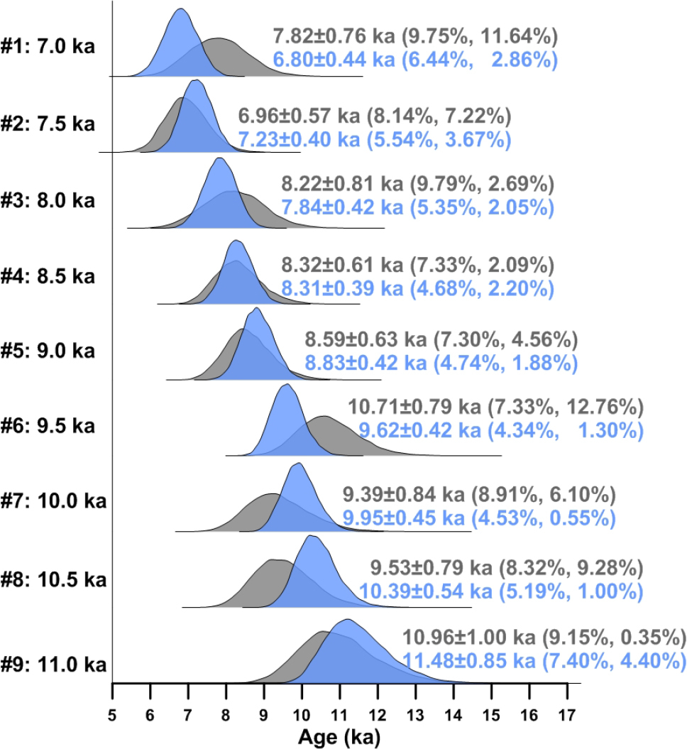
Table 3
A summary of burial dose and age estimated from various statistical age models for nine simulated De sets taken from the same sedimentary sequence. Results obtained using MLE and results obtained using the MCMC sampling protocol as shown in Fig. 2 without and with order constraints are presented. The systematic error on the dose rate measurement shared by all simulated samples was assumed to be σdc=0.
MCMC convergence diagnostics
Although a properly constructed MCMC protocol enables one to draw samples successively from a convergent Markov chain, deciding the point to terminate sampling is sometimes difficult as well as the point to confidently conclude when the algorithm has converged to the desired stationary distribution. One simple and direct way to inspect the convergence of a chain is to check the degree of mixing of the chain by using a trace plot (Fig. 8A). Values that get “stuck” within certain space intervals of variables indicate poor mixing. In contrast, a chain that shows good mixing properties will move freely along the feasible space of variables. Another simple method for assessing the convergence of a chain is to monitor the autocorrelations of generated variables (Fig. 8C). Variables generated using MCMC suffer from autocorrelations to some extent. To decrease the autocorrelations of a variable, simulated samplers are routinely trimmed using a “thinning” protocol after the “burn-in” (“warm-up”) procedure. If the autocorrelations of variables remain extremely high after applying a large “thinning” value, it may imply that the speed of the convergence is slow (i.e., poor mixing) and more samples are therefore needed so that a meaningful inference can be drawn. In this study (unless stated otherwise), the number of “warm-up” iterations per chain was set equal to 2000, and the number of “thinning” iterations per chain was set equal to 1.
Fig. 8
Convergence diagnostics for posterior samples of the CAM burial age from sample GL2-1. The plots were automatically generated using function mcmcSAM(). (A) denotes the trace plot; (B) denotes the density plot; (C) denotes the autocorrelations plot, and (D) denotes the Gelman-Rubin convergence diagnostic plot generated using three parallel Markov chains.
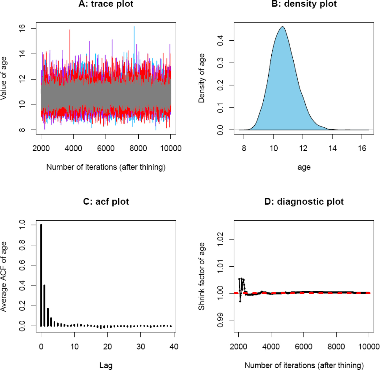
The Gelman-Rubin convergence diagnostic (Gelman and Rubin, 1992) is one of the most widely used methods for monitoring the convergence of MCMC outputs. Several parallel chains are simulated using various initial states when applying this method, and a shrink factor is used as a measurement of the difference between within-chain and between-chain variance (which is similar to the analysis of variance). A shrink factor value equal to or less than 1 indicates adequate convergence, while a factor value significantly above 1 indicates a lack of convergence. Results from Gelman-Rubin convergence diagnostics for posterior samples of CAM burial ages from sample GL2-1 is shown in Fig. 8D. It can be clearly observed that the simulations stabilized and were very close to 1 after approximately 3000 iterations. A summary of Gelman-Rubin convergence diagnostics for sequences of measured and simulated samples obtained using the MCMC sampling protocol of Fig. 2 with order constraints is presented in Table 4.
Table 4
A summary of Gelman-Rubin convergence diagnostics for measured and simulated samples obtained using the MCMC sampling protocol, as shown in Fig. 2 with order constraints. n_eff is the effective sample size, while Rhat (i.e., the shrink factor) is a statistic measure of the ratio of the average variance of samples within each chain to the variance of the pooled samples across chains. If all chains are at equilibrium, the Rhat will be 1. If these chains have not converged to a common distribution, the Rhat statistic will be greater than 1.
. DISCUSSION
This study adopted an MCMC method to obtain sampling distributions on parameters of interest in statistical age models, including the MAM3, CAM, and MXAM3, using De distributions from individual samples and multiple samples with order constraints. It demonstrated that the estimates obtained by MLE and MCMC from measured samples were consistent within errors for various age models (Table 1). In addition, the burial doses and ages obtained by MLE using individual samples and by MCMC using multiple samples simultaneously without order constraints were also broadly consistent between one another (Tables 1–3). These results are encouraging, indicating that the MCMC method potentially provides an alternative perspective for which to analyze statistical age models, and the reliability of parameters of interest can be assessed by comparing the results between the two independent methods (Peng et al., 2016a).
For all MCMC simulations, initial states did not need to be specified and were generated automatically using random number generators, suggesting that the MCMC sampling method employed in this study was not sensitive to the choice of the initial state, and that the algorithm itself was free from the influence of local modes and was able to converge to the desired distribution with a finite number of iterations (Fig. 8 and Table 4). This has a clear advantage over MLE, whereby the latter may result in very different estimates when various starting values are tried, especially for complex age models such as the MAM3, and the MXAM3 (Peng et al., 2013). However, a major drawback of the MCMC method compared to MLE is that a large number of iterations (say, in the tens of thousands) are required in order to explore the entire range of the target distribution, and the process will increasingly be time-consuming given the increase in the number of observations or the complexity of the model under consideration.
When applying the MCMC sampling method to multiple samples with stratigraphic constraints using statistical age models, samples are not analyzed on a standalone basis; rather, they are combined simultaneously in a single model implementation so that between-sample age-depth relationships can also be included. This shows that the burial age of measured samples was internally consistent with the stratigraphy, and the posterior standard deviations of burial ages significantly decreased (Fig. 4). Using simulated De sets with known burial ages demonstrate that the MCMC sampling method can not only increase the precision but also may improve the accuracy of age estimates (Fig. 7). These results illustrate the benefit of including stratigraphic constraints when available during the analysis of statistical age models using De sets from multiple samples (e.g., Cunningham and Wallinga, 2012; Combès and Philippe, 2017). However, it should be noted that incorporating age-depth relationship between samples into the Bayesian model may also have the risk of decreasing the accuracy of age estimates for certain samples within the sequence, as observed in Fig. 7.
The sequence of De sets simulated in Section 4 (Simulated De sets) was determined to be free of systematic error arising from dose rate measurements. However, the systematic error term that induces dependences between observations and the associated age-depth model should always be taken into account when analyzing measured samples (e.g., Rhodes et al., 2003; Combès and Philippe, 2017; Zeeden et al., 2018), although in most cases this error term remains unresolved and subject to guesswork. For example, the systematic error on the dose rate measurement shared by all samples was set to σdc=0.1 for measured samples in this study. The quality of estimates for burial ages may potentially be improved by introducing external (independent) dates, allowing for the correction of systematic components of the error (e.g., Rhodes et al., 2003). This function may be made available in future releases of relevant software programs.
. CONCLUSIONS
This study employed an MCMC sampling method for the statistical analysis of De datasets, using statistical age models, including the CAM, MAM3, and MXAM3. The method was tested using measured, and simulated De sets, and consistent results in agreement with expected values were obtained. The development of numerical programs provides a statistical toolbox for the calculation of OSL ages using MCMC sampling for both individual samples and multiple samples with (or without) order constraints by taking into account systematic and individual errors. The MCMC method employed in this study can be used in addition to other Bayesian models in tackling luminescence-related chronological data and can be flexibly adapted to compute OSL ages of both well- and poorly-bleached sedimentary samples.