. Introduction
The rise in global temperatures since the 20th century has a significant impact on human activities (Esper et al., 2002; Moberg et al., 2005; IPCC, 2014), resulting in temperature changes at both local-regional and global scales, with a strong influence on upland as well as hydrophytic ecosystems (Cao and Woodward, 1998; Shaver et al., 2000). Warming is expected to have significant effects on ecosystems at high latitudes, where plant growth is mainly limited by temperature (Kittel et al., 2000). The Daxing’an Mountains (DM), which are ranging in the northeast across 200–300 km from east to west and extend over 1220 km from south to north, are one of the most sensitive areas to temperature variation of China (Ding et al., 1994; Wang et al., 1998; Zhang et al., 2016). Previous studies showed that temperature change in this region was linked with solar activities and global land-sea atmospheric circulation. The temperature will rise or fall with the intensity or weakness of solar activity (e.g. the warm period in Middle Ages and the cold period in “Little Ice Age”) (Lean and Rind, 1999; Bond et al., 2001; Herrera et al., 2015).
In recent years, the temperature in northeast China has gradually increased, and the temperature in the growing season has risen significantly (Li and Gong, 2006). To understand the potential impacts of climate variation in this region, it is necessary to thoroughly understand the long-term changes and trends of climate over the last hundred years (Esper et al., 2002; Zhang et al., 2003). However, the historical and instrumental meteorological records are very limited before the 1950s. This poses the most significant impediment to comprehending the processes and mechanisms of past climatic fluctuations in this region (Bao et al., 2012). Thus, understanding the characteristics of long-term paleoclimate records are of great research value for the Daxing’an Mountains, which is fundamental for the prediction of future climate.
Over the past few years, the dendrochronological research has made significant progress in China, such as dendroecological research by Song et al., 2011, Yu et al., 2018; dendrogeomorphological research by Malik et al., 2013, 2017. Besides, because the tree-rings are high-resolution climate proxies containing rich climatic information, from which long paleoclimatic records can develop (Shao et al., 2010). This method has been used to extend limited meteorological data and predicts the impacts of various factors over time in various locations around the world (Pederson et al., 2001; Mann et al., 2009; Cook et al., 2010; Davi et al., 2010; Bao et al., 2012; PAGES 2k Consortium, 2013; Pathi et al., 2017). In recent years, some climate reconstruction projects based on tree rings have also been carried out in the northern Greater Khingan Mountains (Liu et al., 2009; Zhang et al., 2011, 2013; Chen et al., 2012; Yu et al., 2012). However, to date, temperature reconstruction based on tree-ring records were still insufficient in the northern Greater Khingan Mountains (Zhang et al., 2013). Thus, this lack must be addressed. Mangui (the site codes MG) is situated in the northern Daxing’an Mountains. A large area of natural temperate old-growth forests in this location provides an excellent opportunity for the study of dendroclimatology, which will allow us to better understand the historical and current climate changes in the northern Daxing’an Mountains region.
This paper uses tree-ring data for Larix gmelinii in Mangui to (1) reconstruct and investigate temperature variability since AD 1880 based on the tree-ring widths from MG, and (2) explore the potential linkages between the reconstructed June-July temperature data and large scale climatic change.
. Materials and methods
Study area and sample collection
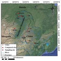
Our study area is located in Mangui in the northern Daxing’an Mountains, Inner Mongolia Autonomous Region, China (Fig. 1). The region experiences a temperate continental monsoon climate, which is characterized by a long and cold winter, windy and dry spring, short and rainy summer, and cool and frosty autumn (Wu et al., 2004). The average annual temperature is −5.7°C, and the annual total precipitation varies from 320 mm to 690 mm, the growing season is from May to September. The slope of the sample site, MG (890 m a.s.l, 52°12’N and 122°17’E), was from 5° to 10°, and the aspect was south. To minimize non-climatic influences on tree growth, the selected stands of Larix gmelinii were naturally established, only healthy Larix gmelinii with no evidence of recent fire, or human disturbance were selected for sampling at breast height. To collect samples that contained consistent climate signals, the elevations difference between the trees of the sample site was within 40 m. One or two tree-ring increment cores were extracted in North-South directions from each tree (In general, two tree cores were taken in each tree, but in some cases, the collected tree core was damaged and discarded, so only one tree core was utilized). In total, 42 cores from 26 Larix gmelinii trees were collected from MG in October 2014.
Fig. 1
Location of the sampling site (MG). Northern Greater Higgnan Mountains (HGHM) (Zhang et al., 2013), Inner Mongolia (IM) (Zhang et al., 2011) and Hulunbuir (HLBE) (Shi et al., 2015) were u asterisk sed for comparison. The cities TH(Tahe), NJ (Nenjiang), NH(Nehe), QQHE(Qiqihar), MX(Maoxing) and HEB (Haerbin) were marked with asterisk.
Development of ring-width chronologies
All cores were preprocessed, air-dried, mounted on the wooden holders using conventional dendrochronological techniques, and subsequently were carefully polished with successively finer grit sandpaper in the laboratory (Fritts, 1976; Holmes, 1983; Cook, 1985). The tree rings were all visually cross-dated with a binocular microscope, annual ring widths were subsequently carefully measured to the nearest 0.001 mm by using a Velmex measuring system. The quality control of cross-dating and measurements was checked by using the COFECHA programme (Holmes, 1983). Each individual ring-width series were detrended in order to remove age-related, non-climatic growth trends (Frits, 1976). A negative exponential curve or straight line was applied to preserve as much low-frequency signal as possible (Cook, 1990). In a few cases, a cubic spline with 67% of the series length was employed when anomalous low-frequency growth trends occurred. The detrended data from individual tree cores were combined into the site chronology by using a bi-weight robust mean method to minimize the influence of extreme values, outliers or bias in tree-ring indices (Cook, 1990). Three kinds of chronologies were generated from ARSTAN: residual (RES), autoregressive (ARS) and standard (STD). The STD chronology was used for further analyses because it includes both low-and high-frequency signals. We limited our analyses to the period with an EPS of at least 0.85 to determine the length of credible chronology (Cook and Briffa, 1990; Wigley et al., 1984).
Climate data
There is no weather station near the sample sites. As such, the interpolated values, based on records from randomly selected 120 of 164 meteorological stations, were used for growth-climate response analysis. (120 weather stations in northeast China were from Chinese Meteorological Data Sharing Service System (http://cdc.cma.gov.cn), another 44 weather stations in Russia from Global Historical Climatology Network (https://www.ncdc.noaa.gov). Meteorological records from a large number of different stations, can reduce the random components or small-scale noise and enhance the reliability of statistical relationships between tree-ring widths and climate data (Pederson et al., 2001).
This interpolation method begins by fitting a partial thin-plate smoothing spline model, that is based on relating location and elevation to ground-based observations to estimate a trend surface, and then a simple kriging procedure was employed to the residuals for trend surface correction (Huang et al., 2013; Li et al., 2014). Analysis of regression was conducted between measured and interpolated precipitations and temperatures at the remaining 44 weather stations, to assess the reliability of the interpolated values. There was a high correlation with R2 = 0.99.
Correlation coefficients between tree-ring width indices and climatic variables from 1959 to 2014 were analyzed by using the data of monthly mean temperature and precipitation. Four climate variables were applied for the dendroclimatological analyses, including monthly total precipitation (Prec), monthly maximum temperature (Tmax), monthly mean temperature (Tmean) and monthly minimum temperature (Tmin). The climate data from the previous June to the current September was used for the correlation analysis.
Global-scale climate variables such as El Niño-Southern Oscillation index (ENSO) and the Pacific Decadal Oscillation index (PDO) (http://climexp.knmi.nl) were also used to assess the tree-ring based climatic signals.
Statistical analyses
Pearson correlation function and growth-climate response analyses (Blasing et al., 1984; Biondi and Waikul, 2004) were utilized to identify the most accepted model for the climatic reconstruction. Subsequently, a simple linear regression equation between the tree-ring width and the climate variables was computed for the calibrated period of 1959–2014. The parameters for calibration and verification included the Pearson’s correlation coefficient (r), explained variance (r2), reduction of error (RE), coefficient of efficiency (CE), sign test (ST) and product means test (PMT). All statistical analyses were performed by using commercial software, SPSS12.0 (SPSS, Inc., Chicago, IL, USA).
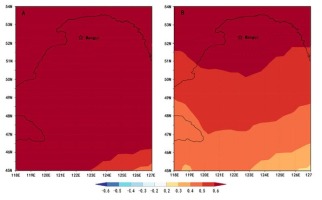
Power spectral analysis was applied to identify reasonable periodicities and performed over the full range of the reconstruction. The spectral properties of the reconstruction series were assessed by using a multi-taper method. In addition, Spatial correlations between the reconstructed Tmean6-7 and the CRU TS 4.01 gridded Tmean dataset (45–52°N, 118–127°E) during the common period of 1960–2013 were analyzed by using the KNMI climate explorer (http://climexp.knmi.nl). This was done to evaluate the spatiotemporal representativeness of the reconstruction.
. Results
Chronology Statistics
The chronology statistics are shown in Table 1. The mean ring width ranged between 0.75 and 1.56 mm. Mean sensitivity (MS), which indicates the relative difference between adjacent rings, was 0.24, reflecting that tree growth was sensitive to the changes of the local environment. The standard deviation (SD) value was 0.26. The first-order autocorrelation among the tree-ring series was 0.60, indicating that tree growth in the current year had a strong influence on growth in the next year (Fritts, 1976). The value of inter-series correlation was 0.60, with a signal-to-noise ratio of 27.60, suggesting that the chronologies recorded adequate environmental signals. The variance in the first eigenvector accounted for 42.0% in the standard chronology. An expressed population signal (EPS) threshold value of 0.85 was used to assess the most credible period of the chronology to ensure the reliability and validity of the reconstruction. The threshold corresponded to a sample depth of three trees and allowed for the reconstruction of the period of 1880–2014.
Table 1
Statistical features of STD chronology.
The relationship between climate and tree-ring width
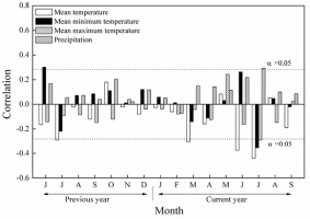
The results of correlation between the MG chronology (STD) and the climatic data revealed that tree-ring width indices were negatively correlated to monthly mean temperatures in almost all months (Fig. 2); the correlations were significant in July of the prior year as well as March and from June to July of the current year (P < 0.05), with the highest correlation coefficient in July of the current year (r = –0.46, P < 0.05) (Fig. 2). Meanwhile, Fig. 2 show there were significant positive correlations between tree-ring index and the June Tmin of the previous year. In addition, Larix gmelinii radial growth in Mangui was positively correlated with precipitation during current June to July, with significant correlation observed in July (Fig. 2). After examining different combinations of months, the best correlation was confirmed between the ring-width indices and monthly mean temperature from current year June to July. Therefore, we reconstructed monthly mean temperature from June to July of the current year by using the MG chronology.
Development of the regression model
Based on the results of correlation analysis, a linear regression model was used in our study to describe the connection between the tree-ring width and the June-July temperatures. The model was designed as follows:
where Tmean6–7 is the mean temperature from June to July of the current year and Xt is the ring-width index of the MG chronology at the t year.
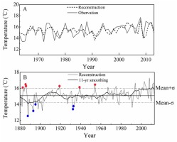
For the calibration period (1959–2014), the reconstruction accounted for 43.6% of the actual Tmean6–7 (Fig. 3), after adjusting for the loss of degrees of freedom, it still explained 42.6% of the total temperature variance. The method of split-sample was employed to check the stability and reliability of the regression model (1) (Liu et al., 2009). Statistics of calibration and verification were shown in Table 3. All calibration and verification parameters were statistically significant (p < 0.05), which indicated that the reconstructed equation was acceptable (Fritts, 1976). In addition, the positive CE and RE values (Table 2) revealed that model (1) was stable and suitable for further temperature reconstruction (Cook et al., 1999). Significant results of PMT and ST showed a good agreement between the reconstructed and actual data. These analyses suggested that the regression model was valid for temperature reconstruction.
Fig. 3
Scatter plot of the tree-ring width index and the averaged Tmean6–7 from June to July (1959–2014).
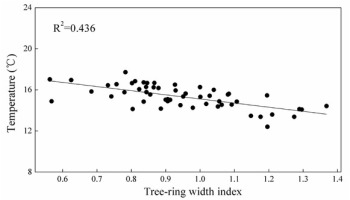
Table 2
Statistics of calibration and verification test for the common period of 1959–2014.
| Calibration | R | R2 | Verification | R | Reduction of error | Coefficient of efficiency | Sign test | Product means test |
|---|---|---|---|---|---|---|---|---|
| Whole section 1959-2014 | 0.66 a | 0.436 a | ||||||
| Front section 1959-1983 | 0.53 a | 0.28 a | Back section 1984–2014 | 0.71a | 0.61a | 0.35a | (26+ /5-) a | 2.8a |
| Back section 1984-2014 | 0.71 a | 0.50 a | Front section 1959–1984 | 0.53a | 0.61a | 0.43a | (21+ / 5-) a | 3.3a |
Table 3
Rank of years of warm/cold reconstructed mean temperature from June to July (Tmean6–7).
Temperature variations from AD 1880 to 2014
Based on model (1), the mean temperature that was reconstructed from 1880 to 2014 for the MG region exhibited a mean of 15.1°C and a standard deviation of σ = 0.88°C. We defined years with values > mean+1σ as a warm year, and values < mean–1σ as a cold year. During the last 134 years, there were 17 warm years, 17 cold years, which accounted for 12.7% of the total reconstruction years, respectively (Table 3). The decadal variability was highlighted by using an 11-year moving average to the reconstruction (Fig. 4B). The warm periods and cold periods can be distinguished. Cold periods occurred in 1887–1898 (average value is 14.2°C), while warm periods occurred in 1994–2014 (15.9°C) (Fig. 4B). Furthermore, there are two obvious processes of mean temperature increasing in 1888–1910 (from 14.1 to 15.5°C, and lasting for 23 years), 1987–2012 (from 15.1 to 16.2°C, and lasting for 26 years).
. Discussion
Tree growth-climate responses
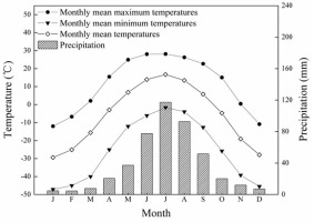
In this study, summer (June to July) temperatures were the most significant negative correlations with the annual radial growth of Larix gmelinii at MG region (Fig. 2). Similar results were also obtained by studies of other tree species in various areas of China (Bao et al., 2012; Gao et al., 2013; Lu et al., 2016; Shi et al., 2013; Tian et al., 2009). The hot summer temperatures might limit the growth of Larix gmelinii due to the increased water deficits caused by the enhanced forest respiration and evaporation of soil moisture (Huang et al., 2010; Zhang et al., 2010). According to the climatic data of the study area from 1959 to 2014, the mean temperature from June to July was significantly negatively correlated with the average precipitation (r = –0.68, P < 0.001), indicating that the effect of precipitation on the growth of Larix gmelinii trees in the high-temperature season was significant. In this study area, soil water is mainly used by trees during the period from June to August, especially in July when the temperature is highest in a year (Bai et al., 2011). The highest precipitation occurs in July-August, but the maximum temperature occurs from June-July (Fig. 5). During this period, the increase in water demand due to transpiration may result in a deficit of soil moisture. Soil moisture evaporation was greater than precipitation, and therefore moisture requirements for growth cannot be met. Our results also revealed that the influence of mean temperatures was more significant than the influence of precipitation during the current June–July. In addition, low temperatures in previous and current June had a great limitation on tree-ring formation. The higher the Tmin in June, the earlier the growth begins, and the longer the growing season, resulting in a wider annual ring (Wu and Shao, 1996). The radial growth of tree rings is affected by the amount of stored compounds. The higher Tmin in June of the previous year may enhance photosynthetic production and store more carbohydrates for the next summer (DeLucia and Smith, 1987). Our results are in line with those of Wang et al., 2005, who suggested that the annual growth of Larix gmelinii trees in Mohe was positively correlated with the Tmin in June, indicating that trees respond to climate with regional homogeneity.
Regional- to large-scale comparison
Drought is not only due to lower precipitation but also to higher temperatures. Under normal rainfall conditions, high temperatures can cause severe droughts, and precipitation is accompanied by low temperatures (Yi et al., 2012; Bao et al., 2012). Historical literature evidence shows that many drought and flooding events occurred in Heilongjiang Province after AD 1880 (Wen and Sun, 2007). The high-temperature years that occurred in AD 1883, 1885, 1886, 1919, 1939, and 1954 were linked with drought events (Table 4) and low-temperature years of 1888, 1892, 1895, 1932 and 1934 were associated with the wet events in the study region (Table 4).
Table 4
The dry/wet years of the reconstructed temperature for the Mangui (MG) region in comparison with historical documents (Wen and Sun, 2007).
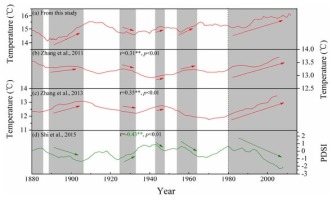
To further evaluate the reliability of this reconstruction, we compared the reconstructed series with nearby tree-ring-based reconstruction temperature series by Zhang et al., 2013 (the site codes NGHM, 680 m a. s. l., 52°55’ N, 121°06’ E; 193 km from our sampling point), Zhang et al., (2011) (the site codes IM, 51°03’15”–52°08’08” N, 120°00’20” – 121°19’21” E; 120 km from our sampling point) and reconstruction Palmer drought severity index (PDSI) series by Shi et al., 2015 (the site codes HLBE, 515–669 m a. s. l., 49°12’ N, 119°42’ E; 607 km from our sampling point) (Fig. 1, Fig. 6). A significant negative correlation (r = –0.43, p < 0.001) between our reconstruction and the May–July PDSI reconstruction in HLBE (Fig. 6d) was found, while our reconstruction of Tmean6–7 had similar variations in the May–October temperature reconstruction in NGHM (r=0.35, p<0.01; Fig. 6c) and May-September temperature reconstruction in IM (r = 0.31, p < 0.01; Fig. 6b). The results showed that despite some differences in these reconstructions, similar temperature patterns were found during 1880–1885, 1888–1906, 1925–1933, 1943–1947, 1953–1964 and 1980–2008 in these areas, (Fig. 6), indicating regional climate change.
Fig. 6
Comparison of June–July mean temperature reconstruction in MG with other tree-ring proxies from surrounding areas: (a) June–July maximum temperature reconstruction in this study; (b) May– September temperature reconstruction in Inner Mongolia (Zhang et al., 2011); (c) May–October temperature reconstruction in northern Greater Higgnan Mountains, China (Zhang et al., 2013); (d) Annual PDSI reconstruction from tree-ring of Mongolian pine in Hulunbuir, Northeast China (Shi et al., 2015). The gray areas mean the common warm/cold periods.
The results showed that the large-scale regional temperature variations had been well captured by our reconstruction, which was significantly positively correlated with regional gridded temperatures (Fig. 7). The above results showed that our reconstruction could capture the temperature signals well. Thus, the reconstruction preserved valid information about regional climate change and provided a valuable profile of past climatic variation in this region.
Possible forcing mechanism
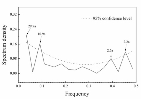
The multi-taper method (MTM) of spectral analysis (Wei, 2010) revealed that the reconstructed Tmean6-7 exhibited significant cycles, which indicated that the Tmean6-7 in MG region could be affected by other factors. Significant peaks of 2.5, and 2.2 years were observed (Fig. 8). The 2–7 years peak cycle was found in some temperature-related reconstruction by tree-rings in the northeast of China (Bao et al., 2012; Liu et al., 2013), which were within the range of the ENSO cycle (Allan et al., 1996; Su and Wang, 2007; Hocke, 2009; Gergis and Fowler, 2009). A possible connection between Tmean6-7 variability and the ENSO was supported by the significantly positive correlations between the reconstructed Tmean6-7 and sea surface temperatures (SSTs) in the eastern equatorial Pacific Ocean (Fig. 9). Some studies have suggested that ENSO had a strong influence on the strength of East Asian Summer Monsoon (EAWM) (Zhang et al., 1999; Wu and Wang, 2002; Lu, 2005). Mangui is located at the boundary zone of the East Asia Summer Monsoon (EASM) (Yang, et al., 1992; Li and Zeng, 2003). The East Asia Summer Monsoon climate regimes dominate the fecundity or deficit of water availability, and trends in temperature (Zhu et al., 2009; Li et al., 2009; Chen et al., 2011, 2012; Gao et al., 2013), the annual warm summers are related to weaker summer East Asia monsoon climate (Zhu et al., 2009; Li et al., 2009). In other words, the stronger the monsoon is, the lower the summer temperature is, and vice versa. The cycles of 10.9-years may suggest the impact of solar effects, such as sunspot activity (Stuiver and Braziunas, 1993; Grootes and Stuiver, 1997; Yi et al., 2012), which was supported by the significant positive correlations of the reconstructed Tmean6–7 with the number of sunspots (http://www.sidc.be/silso/datafiles) from June to July of the current year, with a correlation coefficient of 0.215 (N = 135, 1880–2014, p = 0.009).
Fig. 9
Spatial correlation for the reconstruction with June–July averaged HadlSST1 SST during the period of 1880–2014.
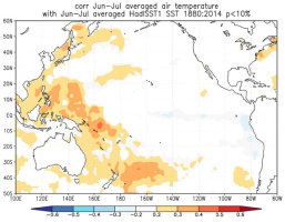
The significant spectral peaks at 29.7-yr (Fig. 8) was possibly linked with the 15–30 yr periods of the Pacific Decadal Oscillation (PDO) (Minobe, 1999; Gedalof et al., 2002; Ma, 2007), which was supported by the significant positive correlations of the reconstructed Tmean6-7 with SSTs in the western Pacific Ocean (Fig. 9) and with the annual PDO (MacDonald and Case 2005), with R2 = 0.156 (N = 117, p < 0.05; 1880–1996). Some other tree-ring studies closed to our study region, discovered that the Hailar pine, Larix gmelinii and tree-ring widths are also significantly correlated with the PDO (Chen et al., 2011, 2012; Bao et al., 2015).
As mentioned above, the complex connections with the ENSO, PDO and Solar activity suggested that the temperature in the Mangui area indicated both local-regional climate signals and global-scale climate changes.
Conclusion
The mean temperature from June to July was reconstructed for the period of 1880 to 2014 by using tree-ring data from MG in the northern Daxing’an Mountains, China. The reconstructed temperature series provided essential information concerning temperature variations in this region. During the last 134 years, there were 17 warm years, 17 cold years, which accounted for 12.7% of the total reconstruction years, respectively. Cold episodes occurred in the intervals 1887–1898, while warm episodes occurred in 1994–2014. In and near the study region, the warmer events coincided with dry periods and the colder events consistent with wet conditions. The spatial correlation analyses between the reconstruction series and gridded temperature data revealed that the regional climatic variations were well captured by this study and the reconstruction represented a regional temperature signal for the northern Daxing’an Mountains. In addition, multi-taper method spectral analysis revealed the existence of significant periodicities in our reconstruction. Significant spectral peaks were found at 29.7, 10.9, 2.5, and 2.2 years. The significant spatial correlations between our temperature reconstruction and the El Niño–Southern Oscillation (ENSO), and Pacific Decadal Oscillation (PDO) and Solar activity suggested that temperature variability in the Mangui area was probably driven by extensive large-scale atmospheric-oceanic variability and solar activity.
